Models

Listen, Attend and Spell (LAS)

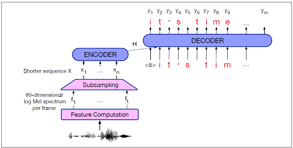
• Attention-based Encoder Decoder (AED)
• The input is a sequence of $t$ acoustic feature vectors $F = f_1, f_2, ..., f_t$, one vector per 10 ms frame
• The output can be letters or wordpieces
• The encoder-decoder architecture is appropriate when input and output sequences have stark length differences: very long acoustic feature sequences mapping to much shorter sequences of letters or words
• Encoder-decoder architecture for speech need to have a compression stage that shortens the acoustic feature sequence before the encoder stage; alternatively use CTC loss function
  • e.g. Low frame rate algorithm: for time $i$, concatenate the acoustic feature vector $f_i$ with the prior two vectors $f_{i-1}, f_{i-2}$

Adding a LM

• Since an encoder-decoder model is essentially a conditional language model, they implicitly learn a language model for the output domain of letters from their training data
• Speech-text datasets are much smaller than pure text datasets
• We can usually improve a model at least slightly by incorporating a very large language model

Beam Search

$score(Y|X) = \frac{1}{|Y|_c} \log{P(Y|X)} + \lambda \log{P_{LM}(Y)}$

• To get a final beam of hypothesized sentences, a.k.a n-best list
• The scoring is done by interpolating the LM score and encoder-decoder score, with a weight $\lambda$ tune on the held-out set
• Since most models prefer shorter sentences, normalize the probability by the number of characters in the hypothesis $|Y|_c$

Connectionist Temporal Classification (CTC)

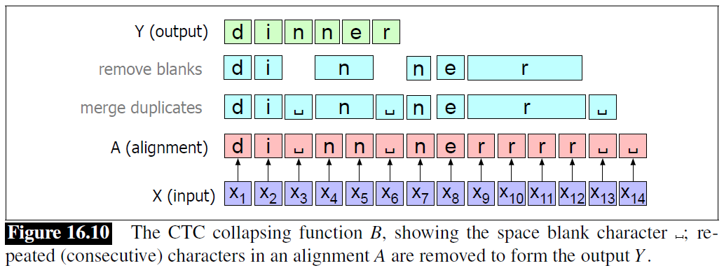
• The intuition of CTC is to output a single character for every frame of the input, so that the output is the same length as the input
• And then to apply a collapsing function that combines sequences of identical letters, resulting in a shorter sequence
• The CTC collapsing function is many-to-one; lots of different alignments map to the same output string

Inference

• The most probable output sequence $Y$ is the one that has, not the single best CTC alignment, but the highest sum over the probability of all its possible alignments:

$P_{CTC}(Y|X) = \sum_{A \in B^{-1}(Y)}{P(A|X)} = \sum_{A \in B^{-1}(Y)}{\prod_{t=1}^{T}{p(a_t|h_t)}}$

$\hat{Y} = \argmax_{Y}{P_{CTC}{(Y|X)}}$

• Because of the strong conditional independence assumption (given the input, the output at time $t$ is independent of the output at time $t-1$), CTC does not implicitly learn a language model
• Essential using CTC to interpolate a language model

Training

The loss for an entire dataset $D$ is the sum of the negative log-likelihoods of the correct output $Y$ for each input $X$:

$L_{CTC} = \sum_{(X,Y) \in D}{-\log{P_{CTC}(Y|X)}}$

RNN-Transducer (RNN-T)

• Because of the strong independence assumption in CTC, recognizers based on CTC don't achieve as high an accuracy as the attention-based encoder-decoder recognizers
• CTC recognizers have the advantage of streaming, recognizing words on-line rather than waiting until the end of the sentence to recognize them
• Removes the conditional independence assumtpion
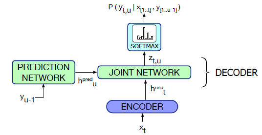
• Two main components: a CTC acoustic model, and a separate language model component called the predictor that conditions on the output token history
• At each time step $t$, the CTC encoder outputs a hidden state $h_{t}^{\text{enc}}$ given the input $x_1 \dots x_t$
• The language model predictor takes as input the previous output token, outputting a hidden state $h_{t}^{\text{pred}}$
• The two hidden states are passed through the joint network, whose output is then passed through a softmax to predict the next character

Tacotron2

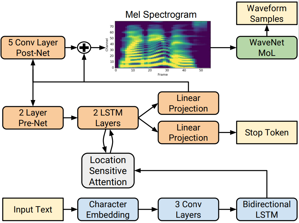
• Extends the earlier Tacotron architecture and the Wavenet vocoder
• An encoder-decoder maps from graphemes to mel spectograms, followed by a vocoder that maps to wavefiles
• Location-based attention, in which the computation of the $\alpha$ values makes use of the $\alpha$ values from the prior time-state
• Autoregressively predict one 80-dimensional log-mel filterbank vector frame (50 ms, with a 12.5 ms stride) at each step
• Stop token prediction, decision about whether to stop producing output
• Trained on gold log-mel filterbank features, using teacher forcing

WaveNet

• An autoregressive network
• Takes spectograms as input and produces output represented as sequences of 8-bit $\mu$-law audio samples
• This means that we can predict the value of each sample with a simple 256-way categorical classifier

The probability of a waveform, a sequence of 8-bit mu-law values $Y = y_1, \dots, y_t$, given an intermediate input mel spectogram $h$ is computed as:

$p(Y) = \prod_{t=1}^{t}{P(y_t | y_1,\dots, y_{t-1}, h_1, \dots, h_t)}$

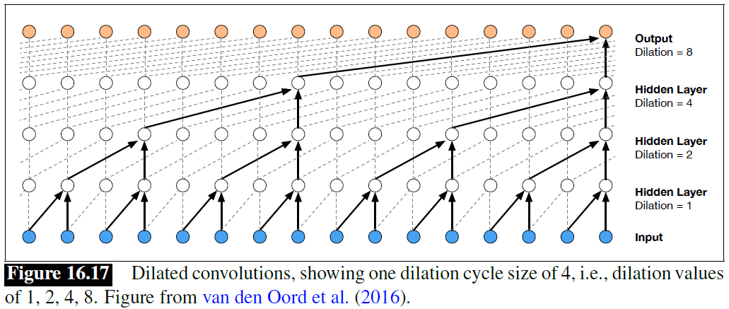
• The probability distribution is modeled by dilated convolution, a subtype of causal convolutional layer
• Dilated convolutions allow the vocoder to grow the receptive field exponentially with depth